How quickly can you debug a CPU performance regression? If your environment is complex and changing quickly, this becomes challenging with existing tools. If it takes a week to root cause a regression, the code may have changed multiple times, and now you have new regressions to debug.
Debugging CPU usage is easy in most cases by using CPU flame graphs. To debug regressions, I would load before and after flame graphs in separate browser tabs, and then blink between them like searching for Pluto. It got the job done, but I wondered about a better way.
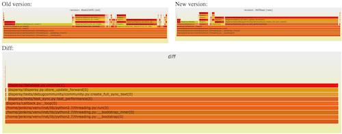
Introducing red/blue differential flame graphs:
This is an interactive SVG (direct link). The color shows red for growth, and blue for reductions.
The size and shape of the flame graph is the same as a CPU flame graph for the second profile (y-axis is stack depth, x-axis is population, and the width of each frame is proportional to its presence in the profile; the top edge is what's actually running on CPU, and everything beneath it is ancestry.)
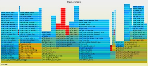
In this example, a workload saw a CPU increase after a system update. Here's the CPU flame graph (SVG):
Normally, the colors are picked at random to differentiate frames and towers. Red/blue differential flame graphs use color to show the difference between two profiles.
The deflate_slow() code and children were running more in the second profile, highlighted earlier as red frames. The cause was that ZFS compression was enabled in the system update, which it wasn't previously.
While this makes for a clear example, I didn't really need a differential flame graph for this one. Imagine tracking down subtle regressions, of less than 5%, and where the code is also more complex.
Red/Blue Differential Flame Graphs
I've had many discussions about this for years, and finally wrote an implementation that I hope makes sense. It works like this:
- Take stack profile 1.
- Take stack profile 2.
- Generate a flame graph using 2. (This sets the width of all frames using profile 2.)
- Colorize the flame graph using the "2 - 1" delta. If a frame appeared more times in 2, it is red, less times, it is blue. The saturation is relative to the delta.
The intent is for use with before & after profiles, such as for non-regression testing or benchmarking code changes. The flame graph is drawn using the "after" profile (such that the frame widths show the current CPU consumption), and then colorized by the delta to show how we got there.
The colors show the difference that function directly contributed (eg, being on-CPU), not its children.
Generation
I've pushed a simple implementation to github (see FlameGraph), which includes a new program, difffolded.pl. To show how it works, here are the steps using Linux perf_events (you can use other profilers).
Collect profile 1:
# perf record -F 99 -a -g -- sleep 30
# perf script > out.stacks1
Some time later (or after a code change), collect profile 2:
# perf record -F 99 -a -g -- sleep 30
# perf script > out.stacks2
Now fold these profile files, and generate a differential flame graph:
$ git clone --depth 1 http://github.com/brendangregg/FlameGraph
$ cd FlameGraph
$ ./stackcollapse-perf.pl ../out.stacks1 > out.folded1
$ ./stackcollapse-perf.pl ../out.stacks2 > out.folded2
$ ./difffolded.pl out.folded1 out.folded2 | ./flamegraph.pl > diff2.svg
difffolded.pl operates on the "folded" style of stack profiles, which are generated by the stackcollapse collection of tools (see the files in FlameGraph). It emits a three column output, with the folded stack trace and two value columns, one for each profile. E.g.:
func_a;func_b;func_c 31 33
[...]
This would mean the stack composed of "func_a()->func_b()->func_c()" was seen 31 times in profile 1, and in 33 times in profile 2. If flamegraph.pl is handed this three column input, it will automatically generate a red/blue differential flame graph.
Options
Some options you'll want to know about:
difffolded.pl -n: This normalizes the first profile count to match the second. If you don't do this, and take profiles at different times of day, then all the stack counts will naturally differ due to varied load. Everything will look red if the load increased, or blue if load decreased. The -n option balances the first profile, so you get the full red/blue spectrum.
difffolded.pl -x: This strips hex addresses. Sometimes profilers can't translate addresses into symbols, and include raw hex addresses. If these addresses differ between profiles, then they'll be shown as differences, when in fact the executed function was the same. Fix with -x.
flamegraph.pl --negate: Inverts the red/blue scale. See the next section.
Negation
While my red/blue differential flame graphs are useful, there is a problem: if code paths vanish completely in the second profile, then there's nothing to color blue. You'll be looking at the current CPU usage, but missing information on how we got there.
One solution is to reverse the order of the profiles and draw a negated flame graph differential. E.g.:
Now the widths show the first profile, and the colors show what will happen. The blue highlighting on the right shows we're about to spend a lot less time in the CPU idle path. (Note that I usually filter out cpu_idle from the folded files, by including a grep -v cpu_idle.)
This also highlights the vanishing code problem (or rather, doesn't highlight), as since compression wasn't enabled in the "before" profile, there is nothing to color red.
This was generated using:
$ ./difffolded.pl out.folded2 out.folded1 | ./flamegraph.pl --negate > diff1.svg
Which, along with the earlier diff2.svg, gives us:
- diff1.svg: widths show the before profile, colored by what WILL happen
- diff2.svg: widths show the after profile, colored by what DID happen
If I were to automate this for non-regression testing, I'd generate and show both side by side.
Update: Elided
Following on from negation, another solution for code paths that vanish in the second profile is to draw them separately as an "elided flame graph." Netflix's internal FlameCommander tool does this. I'll add screenshots when I get a chance, but for now a quick description of how it is presented:
- The red/blue differential flame graph is shown, and on the same page a text string: "X% elided"
- If you click the elided text, it takes you to the elided flame graph
I debated with colleagues (Martin, Jason) about always including the elided flame graph next to the differential flame graph, scaled appropriately. But I realized that most of the time the elided percentage is small, and in those cases the end user may not be very interested in seeing the elided paths. So just the percentage is shown instead and the end user can decide if that's large enough to merit clicking on for the elided flame graph. Not showing it by default helps reduce the number of rectangles to draw and improves browser performance.
CPI Flame Graphs
I first used this code for my CPI flame graphs, where instead of doing a difference between two profiles, I showed the difference between CPU cycles and stall cycles, which highlights what the CPUs were doing.
Other Differential Flame Graphs
There's other ways to do flame graph differentials. Robert Mustacchi experimented with differentials a while ago, and used an approach similar to a colored code review: only the difference is shown, colored red for added (increased) code paths, and blue for removed (decreased) code paths. An example is on the right. It's a good idea, but in practice I found it a bit weird as the frame widths are now the difference only, which is hard to follow without the bigger picture context: a standard flame graph showing the full profile.
Cor-Paul Bezemer has created flamegraphdiff, which shows the difference flame graph along with two standard (bigger picture) flame graphs at the same time: a flame graph for the A and B profiles (before and after). See the example on the right, which has the before and after flame graphs at the top and the difference at the bottom. You can mouse-over frames in the differential, which highlights frames in all profiles. This solves the context problem, since you can see the standard flame graph profiles. I found it a bit slow for complex profiles with many frames, as it is more than doubling the number of rectangles to draw.
My red/blue flame graphs, Robert's hue differential, and Cor-Paul's triple-view, all have their strengths. These could be combined: the top two flame graphs in Cor-Paul's view could be my diff1.svg and diff2.svg. Then the bottom flame graph colored using Robert's approach. For consistency, the bottom flame graph could use the same palette range as mine: blue->white->red.
Flame graphs are spreading, and are now used by many companies. I wouldn't be surprised if there were already other implementations of flame graph differentials I didn't know about. (Leave a comment!)
Conclusion
If you have problems with performance regressions, red/blue differential flame graphs may be the quickest way to find the root cause. These take a normal flame graph and then use colors to show the difference between two profiles: red for greater samples, and blue for fewer. The size and shape of the flame graph shows the current ("after") profile, so that you can easily see where the samples are based on the widths, and then the colors show how we got there: the profile difference.
These differential flame graphs could also be generated by a nightly non-regression test suite, so that performance regressions can be quickly debugged after the fact.
Click here for Disqus comments (ad supported).